|
(If the output comes up as NaN, it means that the number you typed isn't an ordinary non-negative number; there might be a typo in it.)
Most computer languages, and certainly the C language and x86 assembly language come with a built-in square root function. But there are many reasons why we might want to analyze software synthetic methods for computing square roots. One might be for performance reasons either with or without compromises in accuracy, and another is because we might be on a system that simply does not support good performing square roots.
Here is probably the first kind of estimation method (known as the Babylonian method, or Heron's method; however it is easily independently derived by any bright person) that we usually encounter for square roots. We start with an estimate xest for the square root of a value y and iterate it through the following formula:
xest ← (xest + y/xest) / 2
The reasoning behind this is fairly simple. If an estimate xest is too small then y/xest will be too large and vice versa. So we expect that xest < y < y/xest or the other way around and are hoping that the average of the two will become a closer estimate. This is true so long as 0 < xest < y. (However if xest > y, it is easy to show that it will be less than y + 2 in a finite number of iterations, and that it will be less than y/2 + 1/2n after n further iterations.) One can derive this from scratch using Newton's method on the estimation function: f(y, x) = y – x2.
Now, let xest = (√y) * (1 + e). After one iteration we get xest = (√y) * (1 + e2/(2*(1+e))). Thus, for small e, e ← e2 / 2 after each iteration which is better than doubling the number of correct digits or bits after each iteration. That is to say, once the first significant bit is correct, for 53 bits of accuracy, no more than 6 iterations are required. Furthermore, the estimate is always an improvement for any value of e > -1, meaning that any non-zero initial estimate will converge.
The next method we will present here is one that can be used to estimate the square root more incrementally. This is the method usually used when trying to work out square roots by hand, or in certain cases of low accuracy requirements.
Suppose we have an estimate, xest, for the square root of a number y, whose accuracy we measure with the following error function:
err(x,y) = y - xest2
Then we might be interested in the error of a better estimate x+p, err(xest+p,y):
err(xest+p,y)
= y – (xest+p)2
= y – x2 –
2*xest*p – p2
= err(xest,y) –
p*(2* xest + p)
So in an effort to try to make err(x+p,y) as close to 0 as possible, we assume that x is much larger than p and thus solve for p in:
0 = err(xest,y) – p*(2*xest)
which just leads us to p = err(xest,y)/(2*xest). So assuming we can come up with a reasonable initial estimate xest for the square root of y we have a method for iterating this estimate to produce better and better estimates for the square root:
xest is an estimate for y
e = y – xest2
p = e/(2*xest)
e = e – p*(2*xest + p)
xest = xest + p
if xest not close enough go back to step 3
output xest
Now, let xest = √y * (1 + e). After one iteration we get xest = √y * (1 + e2/(2*(1+e))). So it turns out that this is actually the exact same formula as the method given above. The main advantage of this re-expression of this method is that it gives us the opportunity to simplify step 3. For example, if the division in step 3 is only accurate to, say, one digit or bit, then the algorithm will converge exactly one bit or digit per step. So depending on how expensive the division is and how much better we might be able to do with a low accuracy divider, this approach can be better than the first one.
So a simple question is, can we remove the divisions altogether? Ironically, we can, not by estimating the square root, but the reciprocal of the square root (inverse square root). The idea is if we know (1/√y) then y * (1/√y) will give us our desired result. So let us start with an estimate xest of the reciprocal square root and iterate it through the following formula:
xest ← xest*(3 - y*xest2) / 2
This can be derived by plugging the function f(x) = y – 1/x2 into Newton's method. Here we see that if the estimate xest is too small then (3 - y*xest2) will be greater than 2 and if the estimate is too large, then (3 - y*xest2) will be smaller than 2. Unfortunately, we have somewhat tighter requirements on the initial estimate for this to converge successfully. Specifically, we can see that 0 < y*xest2 < 3 is required for it to work.
Now, let xest = (1/√y) * (1 + e). After one iteration we get xest =(1/√y) * (1 – (3/2)*e2 - e3/2). Thus, for small e, e ← -(3/2)*e2 after each iteration which is almost doubling the number of correct digits or bits after each iteration. Although it may require more iterations, the benefit of removing the use of any divisions easily compensates for this.
So how do we get a useful and reliable estimate of 0 < xest< √3/√y without prior access to a square root function?
Well here, fortunately, we can exploit the IEEE-754 format for floating point numbers. Numbers other than 0, inf, -inf, NaN and denormals are represented as:
x = sign * (1 + M) * 2E, 0 ≤ M < 1, E an integer, and sign being -1 or 1.
So we can assume sign is 1, and the square root is basically:
√x = √1 + M * 2(E/2)
So we can plug in a series expansion of (1+x)1/2 to arrive at the following estimate:
√x ≈ (1 + M/2 + O(M2)) * 2floor (E/2) * (1 + (√2-1) * Ind(E is odd))
Now we recall that for small x, 1/(1+x) ≈ 1-x+O(x2), so we can take the reciprocal:
1/√x ≈ (1 - M/2 + O(M2)) * 2 -floor (E/2) * (1 – (1-1/√2) * Ind(E is odd))
The one thing to notice is that this is essentially independent of the exponent magnitude, as far as powers of 2 are concerned. So we need only check this estimate for, say, the range 1 to 4. Between the range 1 and 2-epsilon, the worst deviation is at 2-epsilon which delivers an estimate of 0.5, instead of 0.707... and between the range 2 and 4-epsilon, the worst deviation is at 4-epsilon which delivers an estimate of 0.353 instead of 0.5. This all easily gives us the 0 < xest< √3 / √y we require.
This function is periodic with respect to the exponent but breaks into two distinct cases depending on whether the exponent is even or odd. So lets look at each case one by one. Assuming 1≤x<2 let us consider a slight modification of the formula to:
1/√x ≈ (1 - M/2 + K) * (1/2), for 1≤x<2
Remembering that in this case, x = 1+M, we can plug in the extrema for x and solve for the plausible range of K. This works out to √2-1/2 ≤ K < 1. Now assuming 2≤x<4 we take the additional factor of 2 in the exponent to let x = 2*(1+M). But we will use the same formulaic form as above with a different constant:
1/√x ≈ (1 - M/2 + L) * (1/2), for 2≤x<4
We can again plug in the extrema for x and solve for the plausible range of L. This works out to √2-1 ≤ L < 1/2. This leads us to the observation that K+1/2 ≈ L. So this motivates us to consider a formula of the form:
1/√x ≈ (1 - M/2 + 0.5*Ind(E is even) + L) * 2 -1-floor (E/2)
We should observe that what we have achieved through this reformulation is an expression that is in very nearly the same form as the original IEEE-754 style of number that we started with. In fact let us examine the exact encoding of the IEEE-754 format:
V = [sign (=0)] [biased-exponent (=Bias + E)] [mantissa (= M)]
Notice that the low bit of the biased-exponent appears precisely before the high bit of the mantissa. Thus, a right shift of these bits will:(J - *(unsigned scalar *)&V) >> 1
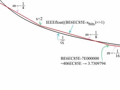
is equivalent to our reformulation (where J is linearly related to the IEEE-754 exponent bias and the value of K or L above). This seems to be a stunning simplification, however by ordering the bits as shown the IEEE-754 specification included consideration into its very design for being able to perform exactly this trick. Solving for J is straight forward and breaks down into the two major cases for 32 bit and 64 bit numbers. First let us take 32 bit numbers, and use the case of 1/√4=0.5. The 32 bit floating point representation of 4 is 0x40800000 (you can use the IEEE-754 format conversion tool here to see this), and the representation of 0.5 is 0x3F000000. This solves to J being 0xBE800000. However, we can take other examples such as 1/√2=0.70710678 and will find that the value of J solves to 0xBE6A09E6. So we can see the rough range for values of J. To find the best J we can scan the range to find the value which causes least deviation from the true inverse square root over the range 1 ≤ x < 4 (or one could use some calculus if sufficiently motivated, but that seems like an excessive effort for what is ultimately going to be an approximation). An example of such a scanner can be downloaded here. This leads to a value of 0xBE6EC85E. Similarly for double precision we find the value of 0xBFCDD90A00000000. The results are accurate to 4 bits, which means at most 4 iterations are required for 32 bit floating point and 5 for 64 bit floating point.
Its time for a graph:
In the standard C programming language one could simply use the standard library function sqrt(). If using another language that does not include a square root function, then the formula sqrt(x) = exp(0.5*ln(x)) can be used. In what follows we will give C and assembly language implementations of the formulas described in the previous section.
Here is a sample C program that implements the third method for 32 bit systems with 64 bit floating point doubles (like the x86):
    double fsqrt (double y) {
    double x, z, tempf;
    unsigned long *tfptr = ((unsigned long *)&tempf) + 1;

	tempf = y;
	*tfptr = (0xbfcdd90a - *tfptr)>>1; /* estimate of 1/sqrt(y) */
	x =  tempf;
	z =  y*0.5;                        /* hoist out the “/2”    */
	x = (1.5*x) - (x*x)*(x*z);         /* iteration formula     */
	x = (1.5*x) – (x*x)*(x*z);
	x = (1.5*x) – (x*x)*(x*z);
	x = (1.5*x) – (x*x)*(x*z);
	x = (1.5*x) – (x*x)*(x*z);
	return x*y;
    }
As a further optimization, only the top 32bits are manipulated for the estimate, and the iteration formula is just unrolled to some arbitrary degree. The parentheses in the iteration formula will cause the compiler to build code which performs well on processors which support pipelined floating point operations (and out-of-order execution). Here is a similar program written in inline assembly language (for the MSVC compiler):
    /* Copyright (C) 1997 by Vesa Karvonen. All rights reserved.
    **
    ** Use freely as long as my copyright is retained.
    */

    double __stdcall Inv_Sqrt(double x) {
    __asm {
    ; I'm assuming that the argument is aligned to a 64-bit boundary.

        mov     eax,0BFCDD6A1h  ; 1u    Constant from James Van Buskirk
        mov     edx,[esp+8]     ; 1v    Potential pms.
        sub     eax,edx         ; 2u
        push    03FC00000h      ; 2v    Constant 1.5, aligns stack
        shr     eax,1           ; 3u
        sub     edx,000100000h  ; 3v    =.5*x, biased exponent must > 1
        mov     [esp+12],edx    ; 4u
        push    eax             ; 4v

    ; The lower 32-bits of the estimate come from uninitialized stack.

        fld     QWORD PTR [esp-4]   ; 5     Potential pms
        fmul    st,st               ; 6-8
        fld     QWORD PTR [esp-4]   ; 7
        fxch    st(1)               ; 7x
        fmul    QWORD PTR [esp+12]  ; 9-11  Potential pms
        fld     DWORD PTR [esp+4]   ; 10
        add     esp,4               ; 12    Faster on Pro/PII
        fsub    st,st(1)            ; 12-14

        fmul    st(1),st        ; 15-17
        fmul    st(1),st        ; 18-20
        fld     DWORD PTR [esp] ; 19
        fxch    st(1)           ; 19
        fmulp   st(2),st        ; 20-22
        fsub    st,st(1)        ; 21-23

        fmul    st(1),st        ; 24-26
        fmul    st(1),st        ; 27-29
        fld     DWORD PTR [esp] ; 28
        fxch    st(1)           ; 28
        fmulp   st(2),st        ; 29-31
        fsub    st,st(1)        ; 30-32

        fmul    st(1),st        ; 33-35
        pop     eax             ; 34
        fmul    st(1),st        ; 36-38
        fld     DWORD PTR [esp] ; 37
        fxch    st(1)           ; 37
        fmulp   st(2),st        ; 38-40
        fsubrp  st(1),st        ; 39-41
        fmulp   st(1),st        ; 42-44
    }
    }
It should also be pointed out that these methods will not get exactly rounded answers – they are approximations. These techniques are all well known to CPU and compiler vendors, and thus one cannot expect to directly outperform, or be more accurate than C library's sqrt() function. However, by deriving these functions we are able to easily create estimations that deliver lower accuracy yet with higher performance than could be delivered by standard libraries or CPU microcode which are required to deliver accurate answers.
In general, for full floating point approximations, the first two methods are slower than the third given in the above in practical implementations. Our next task is to look at few simple cases where simplification is very important.
	; invsqrt2 computes an approximation to the inverse square root of an
	; IEEE-754 single precision number. The algorithm used is that
	; described in this paper: Masayuki Ito, Naofumi Takagi, Shuzo Yajima:
	; "Efficient Initial Approximation for Multiplicative Division
	; and Square Root by a Multiplication with Operand Modification". IEEE
	; Transactions on Computers, Vol. 46, No. 4, April 1997,
	; pp 495-498.
	;
	; This code delivers inverse square root results that differ by at most 1
	; ulp from correctly rounded single precision results. The correctly
	; rounded single precision result is returned for 99% of all arguments
	; if the FPU precision is set to either extended precision (default under
	; DOS) or double precision (default under WindowsNT). This routine does
	; not work correctly if the input is negative, zero, a denormal, an
	; infinity or a NaN. It works properly for arguments in [2^-126, 2^128),
	; which is the range of positive, normalized IEEE single precision numbers
	; and is roughly equivalent to [1.1755e-38,3.4028e38].
	;
	; In case all memory accesses are cache hits, this code has been timed to
	; have a latency of 39 cycles on a PentiumMMX.
	;
	;
	; invsqrt2 - compute an approximation to the inverse square root of an
	;            IEEE-754 single precision number.
	;
	; input:
	;    ebx  = pointer to IEEE-754 single precision number, argument
	;    esi  = pointer to IEEE-754 single precision number, res = 1/sqrt(arg)
	;
	; output:
	;   [esi] = 1/sqrt(arg)
	;
	; destroys:
	;   eax, ecx, edx, edi
	;   eflags
	;

	INVSQRT2 MACRO

	         .DATA

	d1tab    dw      0B0DDh,0A901h,0A1B5h,09AECh,0949Ah,08EB2h,0892Ch,083FFh
	         dw      07E47h,07524h,06C8Ah,0646Eh,05CC6h,05589h,04EAFh,04831h
	         dw      04208h,03C2Fh,0369Fh,03154h,02C49h,0277Ah,022E3h,01E81h
	         dw      01A51h,0164Fh,01278h,00ECBh,00B45h,007E3h,004A3h,00184h
	         dw      0FA1Fh,0EF02h,0E4B1h,0DB18h,0D227h,0C9CEh,0C1FEh,0BAACh
	         dw      0B3CDh,0AD57h,0A742h,0A186h,09C1Ch,096FEh,09226h,08D8Fh
	         dw      08934h,08511h,08122h,07AC7h,073A6h,06CD9h,0665Ch,06029h
	         dw      05A3Ch,05491h,04F24h,049F1h,044F4h,0402Ch,03B94h,0372Ah

	half     ds      0.5
	three    ds      3.0

	         .CODE

	         mov     eax, [ebx]       ; arg (single precision floating-point)
	         mov     ecx, 0be7fffffh  ; 0xbe7fffff
	         mov     edi, eax         ; arg
	         mov     edx, eax         ; arg
	         shr     edi, 18          ; (arg << 18)
	         sub     ecx, eax         ; (0xbe7fffff - arg)
	         shr     eax, 1           ; (arg << 1)
	         and     edi, 3fh         ; index = ((arg << 18) & 0x3f)
	         shr     ecx, 1           ; ((0xbe7fffff - arg) << 1)
	         and     eax, 00001ffffh  ; (arg << 1) & 0x1ffff
	         movzx   edi, d1tab[edi*2]; d1tab[index]
	         and     edx, 0007e0000h  ; arg & 0x7e0000
	         and     ecx, 07f800000h  ; exo=((0xbe7fffff - arg) <1) & 0x7f800000
	         or      eax, edx         ; (arg & 0x7e0000) | ((arg <1) & 0x1fff)
	         shl     edi, 8           ; d1tab[index] >> 8
	         xor     eax, 00002ffffh  ; (arg&0x7e0000)|((arg<<1)&0x1fff)^0x2ffff
	         add     edi, 03f000000h  ; d1 = (d1tab[index] >> 8) | 0x3f000000
	         or      eax, ecx         ; xhat = ((arg&0x7e0000)|((arg<<1)&0x1fff)^0x2ffff)|expo
	         push    edi              ; d1
	         push    eax              ; xhat
	         fld     dword ptr [esp+4]; d1
	         fmul    dword ptr [esp]  ; approx = d1*xhat
	         fld     st(0)            ; approx approx
	         fmul    st,st(0)         ; approx*approx approx
	         fxch    st(1)            ; approx approx*approx
	         fmul    dword ptr [half] ; approx*0.5 approx*approx
	         fxch    st(1)            ; approx*approx approx*0.5
	         fmul    dword ptr [ebx]  ; approx*approx*arg approx*0.5
	         fsubr   dword ptr [three]; 3-approx*approx*arg approx*0.5
	         fmulp   st(1),st         ; res = (3-approx*approx*arg)*approx*0.5
	         fstp    dword ptr [esi]  ; store result
	         add     esp,8            ; remove floating-point temps
	ENDM
Some sample code from nVidia corporation suggests that in fact table look ups alone might be a plausible approach. You can see their code here. Their code also includes reciprocal approximation code. However this table is very large and thus utilizing your cache for this purpose will mean it is less utilized for other purposes. I.e., it may really just transfer the penalty of a cache miss to some other part of your code. Note that the price of a cache miss in modern processors is much higher than using non-memory based methods such as the ones described here or using the processors built-in mechanism for computing square roots. Of course, with the advent of SIMD instruction sets in modern x86 CPUs, some of these approximations have been incorporated into the instruction set itself. The following is an example that computes two parallel inverse square roots using AMD's 3DNow! instruction set which was introduced in 1997:
	.586
	.MMX
	.K3D

	MOVQ		MM0, [mem]	;         b | a
	PFRSQRT         MM1, MM0 	; 1/sqrt(a) | 1/sqrt(a) (12 bit approx)
	MOVQ            MM2, MM0	;
	PUNPCKHDQ       MM0, MM0	;         b | b
	PFRSQRT         MM0, MM0        ; 1/sqrt(b) | 1/sqrt(b) (12 bit approx)
	PUNPCKLDQ       MM1, MM0        ; 1/sqrt(b) | 1/sqrt(a) (12 bit approx)
	MOVQ            MM0, MM1	;
	PFMUL           MM1, MM1	;      ~1/b | ~1/a      (12 bit approx)
	PFRSQIT1        MM1, MM2        ;       ??? | ???
	PFRCPIT2        MM1, MM0	; 1/sqrt(b) | 1/sqrt(a) (23 bit approx)
Which, of course, will give the highest throughput of any of the code shown here, but is tied to a particular processor architecture.
When integer outputs are required, the first two methods become more sensible choices. Let us first look at integer output for an integer input of square root (i.e., computing (int)sqrt((int)x);)
The following is a fairly fast implementation using the first method:
	/*
	// Integer Square Root function
	// Contributors include Arne Steinarson for the basic approximation idea,
	// Dann Corbit and Mathew Hendry for the first cut at the algorithm,
	// Lawrence Kirby for the rearrangement, improvments and range optimization
	// and Paul Hsieh for the round-then-adjust idea.
	*/
	static unsigned fred_sqrt(unsigned long x) {
	    static const unsigned char sqq_table[] = {
	       0,  16,  22,  27,  32,  35,  39,  42,  45,  48,  50,  53,  55,  57,
	      59,  61,  64,  65,  67,  69,  71,  73,  75,  76,  78,  80,  81,  83,
	      84,  86,  87,  89,  90,  91,  93,  94,  96,  97,  98,  99, 101, 102,
	     103, 104, 106, 107, 108, 109, 110, 112, 113, 114, 115, 116, 117, 118,
	     119, 120, 121, 122, 123, 124, 125, 126, 128, 128, 129, 130, 131, 132,
	     133, 134, 135, 136, 137, 138, 139, 140, 141, 142, 143, 144, 144, 145,
	     146, 147, 148, 149, 150, 150, 151, 152, 153, 154, 155, 155, 156, 157,
	     158, 159, 160, 160, 161, 162, 163, 163, 164, 165, 166, 167, 167, 168,
	     169, 170, 170, 171, 172, 173, 173, 174, 175, 176, 176, 177, 178, 178,
	     179, 180, 181, 181, 182, 183, 183, 184, 185, 185, 186, 187, 187, 188,
	     189, 189, 190, 191, 192, 192, 193, 193, 194, 195, 195, 196, 197, 197,
	     198, 199, 199, 200, 201, 201, 202, 203, 203, 204, 204, 205, 206, 206,
	     207, 208, 208, 209, 209, 210, 211, 211, 212, 212, 213, 214, 214, 215,
	     215, 216, 217, 217, 218, 218, 219, 219, 220, 221, 221, 222, 222, 223,
	     224, 224, 225, 225, 226, 226, 227, 227, 228, 229, 229, 230, 230, 231,
	     231, 232, 232, 233, 234, 234, 235, 235, 236, 236, 237, 237, 238, 238,
	     239, 240, 240, 241, 241, 242, 242, 243, 243, 244, 244, 245, 245, 246,
	     246, 247, 247, 248, 248, 249, 249, 250, 250, 251, 251, 252, 252, 253,
	     253, 254, 254, 255
	    };

	    unsigned long xn;

	    if (x >= 0x10000)
	        if (x >= 0x1000000)
	            if (x >= 0x10000000)
	                if (x >= 0x40000000) {
	                    if (x >= 65535UL*65535UL)
	                        return 65535;
	                    xn = sqq_table[x>>24] << 8;
	                } else
	                    xn = sqq_table[x>>22] << 7;
	            else
	                if (x >= 0x4000000)
	                    xn = sqq_table[x>>20] << 6;
	                else
	                    xn = sqq_table[x>>18] << 5;
	        else {
	            if (x >= 0x100000)
	                if (x >= 0x400000)
	                    xn = sqq_table[x>>16] << 4;
	                else
	                    xn = sqq_table[x>>14] << 3;
	            else
	                if (x >= 0x40000)
	                    xn = sqq_table[x>>12] << 2;
	                else
	                    xn = sqq_table[x>>10] << 1;

	            goto nr1;
	        }
	    else
	        if (x >= 0x100) {
	            if (x >= 0x1000)
	                if (x >= 0x4000)
	                    xn = (sqq_table[x>>8] >> 0) + 1;
	                else
	                    xn = (sqq_table[x>>6] >> 1) + 1;
	            else
	                if (x >= 0x400)
	                    xn = (sqq_table[x>>4] >> 2) + 1;
	                else
	                    xn = (sqq_table[x>>2] >> 3) + 1;

	            goto adj;
	        } else
	            return sqq_table[x] >> 4;

	/* Run two iterations of the standard convergence formula */

	    xn = (xn + 1 + x / xn) / 2;
	nr1:
	    xn = (xn + 1 + x / xn) / 2;
	adj:

	    if (xn * xn > x) /* Correct rounding if necessary */
	       xn--;

	    return xn;
	}
This version is rounded to exactly the correct result (a likely desire for
integer parameters). However, we can see that the code is dominated by
unpredictable branches. For modern CPUs this has the problem of taxing the
branch predictors which are likely to perform less than optimally on this
code. The following is code more suited to deeply pipelined processors with
fast FPUs (it requires that longs are 32 bits, and that the FPU supports
IEEE-754 32 bit floats):
	int isqrt (long r) {
	    float tempf, x, y, rr;
	    int is;

	    rr = (long) r;
	    y = rr*0.5;
	    *(unsigned long *) &tempf = (0xbe6f0000 - *(unsigned long *) &rr) >> 1;
	    x = tempf;
	    x = (1.5*x) - (x*x)*(x*y);
	    if (r > 101123) x = (1.5*x) - (x*x)*(x*y);
	    is = (int) (x*rr + 0.5);
	    return is + ((signed int) (r - is*is)) >> 31;
	}
Let us examine an implementation of the second method:
	/* by Jim Ulery */
	static unsigned julery_isqrt(unsigned long val) {
	    unsigned long temp, g=0, b = 0x8000, bshft = 15;
	    do {
	        if (val >= (temp = (((g << 1) + b)<<bshft--))) {
	           g += b;
	           val -= temp;
	        }
	    } while (b >>= 1);
	    return g;
	}
Here the division step is replaced with a 1-bit approximation of that
division. Jim Ulery's complete
derivation is given here. But there are still 15 branches here that will
not be predicted very well, as well as loop overhead. So unrolling is the
first improvement we can make:
	/* by Mark Crowne */
	static unsigned int mcrowne_isqrt (unsigned long val) {
	  unsigned int temp, g=0;

	  if (val >= 0x40000000) {
	    g = 0x8000;
	    val -= 0x40000000;
	  }

	#define INNER_ISQRT(s)                        \
	  temp = (g << (s)) + (1 << ((s) * 2 - 2));   \
	  if (val >= temp) {                          \
	    g += 1 << ((s)-1);                        \
	    val -= temp;                              \
	  }

	  INNER_ISQRT (15)
	  INNER_ISQRT (14)
	  INNER_ISQRT (13)
	  INNER_ISQRT (12)
	  INNER_ISQRT (11)
	  INNER_ISQRT (10)
	  INNER_ISQRT ( 9)
	  INNER_ISQRT ( 8)
	  INNER_ISQRT ( 7)
	  INNER_ISQRT ( 6)
	  INNER_ISQRT ( 5)
	  INNER_ISQRT ( 4)
	  INNER_ISQRT ( 3)
	  INNER_ISQRT ( 2)

	#undef INNER_ISQRT

	  temp = g+g+1;
	  if (val >= temp) g++;
	  return g;
	}
Dropping to inline assembly language (for MSVC) again, we can replace the branch code with conditional computation:
	/* by Norbert Juffa */
	__declspec (naked) unsigned long __stdcall isqrt (unsigned long x) {
	/* based on posting by Wilco Dijkstra in comp.sys.arm in 1996 */
	#define iter(N)               \
	  trial = root2 + (1 << (N)); \
	  foo = trial << (N);         \
	  if (n >= foo) {             \
	    n -= foo;                 \
	    root2 |= (2 << (N));      \
	  }

	/*
	 * For processors that provide single cycle latency
	 * LEA, the first four instructions of the following
	 * macro could be replaced as follows
	 * __asm   lea    edx, [eax+(1<<(N))]
	 * __asm   lea    ebx, [eax+(2<<(N))]
	 */
	#if CPU == ATHLON || CPU == ATHLON64
	#define iterasm(N) \
	  __asm   mov    edx, (1 << (N))  \
	  __asm   mov    ebx, (2 << (N))  \
	  __asm   or     edx, eax         \
	  __asm   or     ebx, eax         \
	  __asm   shl    edx, (N)         \
	  __asm   mov    esi, ecx         \
	  __asm   sub    ecx, edx         \
	  __asm   cmovnc eax, ebx         \
	  __asm   cmovc  ecx, esi
	#else /* generic 386+ */
	#define iterasm(N) \
	  __asm   mov    edx, (1 << (N))  \
	  __asm   mov    ebx, (2 << (N))  \
	  __asm   or     edx, eax         \
	  __asm   or     ebx, eax         \
	  __asm   shl    edx, (N)         \
	  __asm   sub    ecx, edx         \
	  __asm   sbb    esi, esi         \
	  __asm   sub    eax, ebx         \
	  __asm   and    eax, esi         \
	  __asm   add    eax, ebx         \
	  __asm   and    edx, esi         \
	  __asm   add    ecx, edx
	#endif

	  __asm {
	    mov    ecx, [esp+4] ; x
	    push   ebx          ; save as per calling convention
	    push   esi          ; save as per calling convention
	    xor    eax, eax     ; 2*root
	    /* iteration 15 */
	    mov    ebx, (2 << (15))
	    mov    esi, ecx
	    sub    ecx, (1 << (30))
	    cmovnc eax, ebx
	    cmovc  ecx, esi
	    iterasm (14);
	    iterasm (13);
	    iterasm (12);
	    iterasm (11);
	    iterasm (10);
	    iterasm (9);
	    iterasm (8);
	    iterasm (7);
	    iterasm (6);
	    iterasm (5);
	    iterasm (4);
	    iterasm (3);
	    iterasm (2);
	    iterasm (1);
	    /* iteration 0 */
	    mov    edx, 1
	    mov    ebx, 2
	    add    edx, eax
	    add    ebx, eax
	    sub    ecx, edx
	    cmovnc eax, ebx
	    shr    eax, 1
	    mov    esi, [esp]   ; restore as per calling convention
	    mov    ebx, [esp+4] ; restore as per calling convention
	    add    esp, 8       ; remove temp variables
	    ret    4            ; pop one DWORD arg and return
	  }
	}
(Note that although other x86 processors can execute cmovCC instructions,
they do not yield improvements in performance over the code given except on
Athlon based processors.) This solution significantly outperforms the first
method.
Norbert wrote in to inform me that cmovCC, sbb and setCC instructions are
intolerably slow on the P4 platform. However:
|
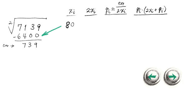
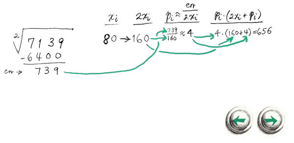
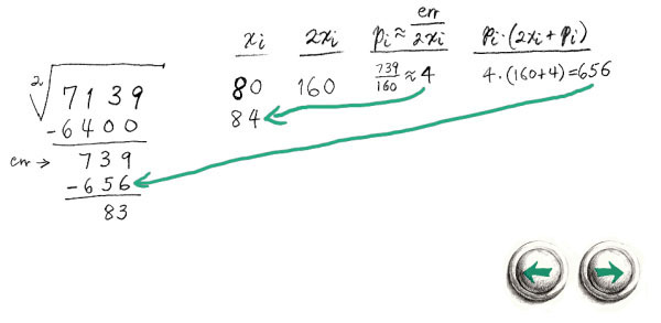
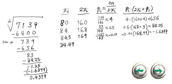
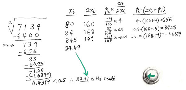
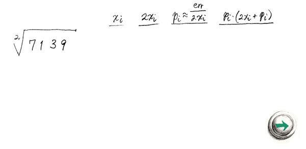
And now to satisfy an interesting comment by Carl Sagan. In his book, The Demon Haunted World the famous astronomer decried the fact that in public school he learned a method for calculating square roots by hand, without knowing how or why it worked. Well, we've already explained the key method, namely the second approximation method described in section 1. So we will perform a “quick division” at step 3, by simply performing 1-digit approximations so that we can simplify our calculations. For the other calculations we need a few columns of scratch space. Let us start with an example of a square root performed by hand:
Click on the navigation buttons to follow each step. To understand how each step was arrived at, follow the arrows to see the order the calculations. If you were taught a square root by hand method in school, you may note that it is a little different than this method. One inefficiency I have always found about long division, and square root methods taught in school is that they are intolerant of over-estimations. But sometimes over-estimations can get you much closer to the answer. Usually subtracting from an overestimate is easier than restricting your calculations to underestimates. This can make the termination, and rounding steps more complicated, but this is usually made up for by simpler intermediate calculations. For integers, the termination condition is when err < 0.5. This ensures that the square of the result gives the correctly rounded result.
See also Extracting Square Roots by means of the Napier rodsA common application in computer graphics, is to work out the distance between two points as √(Δx2+Δy2). However, for performance reasons, the square root operation is a killer, and often, very crude approximations are acceptable. So we examine the metrics (1 / √2)*(|x|+|y|), and max(|x|,|y|):
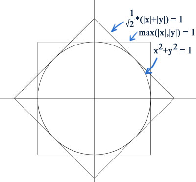
Notice the octagonal intersection of the area covered by these metrics, that very tightly fits around the ordinary distance metric. The metric that corresponds to this, therefore is simply:
octagon(x,y) = min ((1 / √2)*(|x|+|y|), max (|x|, |y|))
With a little more work we can bound the distance metric between the following pair of octagonal metrics:
octagon(x,y) / (4-2*√2) ≤ √(x2+y2) ≤ octagon(x,y)
Where 1/(4-2*√2) ≈ 0.8536, which is not that far from 1. So we can get a crude approximation of the distance metric without a square root with the formula:
distanceapprox (x, y) = (1 + 1/(4-2*√2))/2 * min((1 / √2)*(|x|+|y|), max (|x|, |y|))
which will deviate from the true answer by at most about 8%. A similar derivation for 3 dimensions leads to:
distanceapprox (x, y, z) = (1 + 1/4√3)/2 * min((1 / √3)*(|x|+|y|+|z|), max (|x|, |y|, |z|))
with a maximum error of about 16%.
However, something that should be pointed out, is that often the distance is only required for comparison purposes. For example, in the classical mandelbrot set (z←z2+c) calculation, the magnitude of a complex number is typically compared to a boundary radius length of 2. In these cases, one can simply drop the square root, by essentially squaring both sides of the comparison (since distances are always non-negative). That is to say:
√(Δx2+Δy2) < d is equivalent to Δx2+Δy2 < d2, if d ≥ 0These are probably the most relevant rules about square roots in ordinary mathematical calculations:
√a*b = √a
*√b, if a,b ≥ 0
ln√a = (½)*ln(a), if a > 0
√1/a = 1/√a, if a > 0
√(a2) = |a|
(√a)2 = a, if a ≥ 0
1/(√a+√b) = (√a-√b)/(a-b), if a,b ≥ 0, a≠b
1/(√a-√b) = (√a+√b)/(a-b), if a,b ≥ 0, a≠b
|a + i*b| = √(a2+b2)
Where a and b are real numbers and the domain restrictions are given (and cannot be ignored). The square root of a complex number can be computed as:
√a+i*b = ±√((√(a2+b2)+a)/2) ± i*√((√(a2+b2)-a)/2)
Note that the signs for each component needs to be selected correctly. That is to say, only two of the four possible choices are correct. If b > 0 the signs must be the same. If b < 0 the signs must be different. If b = 0, then only one of the components is nonzero and can be either sign. The above is not a definition, but rather just a way of calculating a value whose square gives the original.
As a matter of history, square roots, are interesting in that they introduced “irrational numbers” to Pythagoras (~570 - 500 BCE), who had thought that all numbers were expressible as a fraction (a rational.) One of his disciples, Hippasus, however using a method called “reducto ad absurdum” (aka proof by contradiction) discovered that in fact there were numbers that could not be expressed as a fraction:
Suppose x/y = √2, where x and y are integers. Then x2 = 2*y2. But then the LHS has an even number of factors of 2, while the RHS has an odd number of factors of 2. This is impossible, therefore the original assumption that there exists integers x and y such that x/y = √2 must be false. QED.
This all happened at a time before the idea of academic research and the promotion of open discussion of mathematics was pervasive. The Pythagoreans were, in fact, a kind of cult. The knowledge of mathematics and other secrets where known only to those in the inner circle. Before this discovery, Pythagoras and his followers proselytized to farmers and other people interested in calculations at the time that all numbers could be expressed as rationals. When the Pythagoreans discovered the existence of non-rationals, they decided to withhold it from the public and kill Hippasus for his discovery.
Square roots continued to be important to Pythagoras, of course, as a method for calculating right triangle edge lengths from Pythagoras' theorem (though there is strong evidence that the Babylonians were already aware of this prior to Pythagoras).
We know, because of YBC 7289 (1800 - 1600 BCE), that the Babylonians knew about square roots. On YBC 7289 is a depiction of a square and its diagonals shown with ancient cuneiform writing depicting the fraction: 1 + 24/60 + 51/602 + 10/603 which is the closest approximation to √2 available to that level (4 base 60 digits) of accuracy. Stephen K Stephenson has a video demonstration of exactly how they are likely to have calculated it using Heron's method and counting stones. Part 1 Part 2 Part 3 The point of the video(s), I think, is to demonstrate how the Babylonians could have practically calculated √2 without the use of calculators, or pencils and paper (they had clay and reeds; wax tablets had not yet been invented.)
Pythagoras' theorem eventually lead to the 17th century French number theorist Pierre de Fermat to ponder variations of the same equation with powers higher than two. Fermat's statement that xn+yn=zn has no non-trivial integer solutions for n>2 (better known as Fermat's last theorem), was not finally settled as true until 1995 by the English Mathematician Andrew Wiles.